Page 84 - ITU Journal, Future and evolving technologies - Volume 1 (2020), Issue 1, Inaugural issue

ITU Journal on Future and Evolving Technologies, Volume 1 (2020), Issue 1

informing an available user. API Callback:
(HSF type, Impinging wave, R equired departing wavefront)
5. THE METAMATERIAL MIDDLE-
Phased array model Neural network
WARE Workflow model equivalent rays model
Phased array + circuit
For the metamaterial to be reconfigured between dif- equivalent model Raw EM field model
ferent functionalities, a physical mechanism for locally Analytical model-
based initial
tuning each unit cell response must be infused [8]. In the solution Period bounds
context of the present work, we assume that the response detection
of the unit cells is controlled by variable impedance loads Smart solution- Effective variable
connected to the front side metallization layer of the space reduction discretization
Goodness-of-Fit
metamaterial, where structures such as the resonant metric Physics-derived
patch pair resides [3]. The loads are complex valued Model-based variable restrictions
Regression calibration
variables, comprising resistors and capacitors or induc- Approach (XCSF)
tors. The value of the i-th load, Z i = R i + jX i , com- Optimization engine
prises two parameters: its resistance (R i > 0) and re- selection & initialization
actance (X i = −(ωC i ) −1 or X i = +ωL i ), for capacitive
and inductive loads, respectively. The loads are, thus, Simulations-driven Fitness Function
electromagnetically connected to the surface impedance Optimization Loop
of the “unloaded” unit cell and by tuning their values Measurements-driven Machine learning-
based accelerator
we can regulate the unit cell response, e.g. the ampli-
tude and phase of its reflection coefficient. The latter is
Store optimal (Populate training
naturally a function of frequency and incoming ray di- configuration to DB dataset)
rection and polarization. When the metamaterial unit
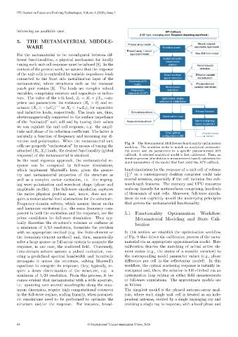
Fig. 9 – The Metamaterial Middleware functionality optimization
cells are properly “orchestrated” by means of tuning the workflow. The workflow seeks to match an analytical metamate-
attached (R i , X i ) loads, the desired functionality (global rial model and its parameters to a specific parameterized API
response) of the metamaterial is attained. callback. A selected analytical model is first calibrated. Then, an
iterative process (simulation or measurement-based) optimizes the
In the most rigorous approach, the metamaterial re-
input parameters of the model that best yield the API callback.
sponse can be computed by full-wave simulations,
which implement Maxwell’s laws, given the geome- band simulation for the response of a unit cell of volume
λ 3
try and metamaterial properties of the structure as ( ) on a contemporary desktop computer could take
5
well as a complex vector excitation, i.e. the imping- several minutes, especially if the cell includes fine sub-
ing wave polarization and wavefront shape (phase and wavelength features. The memory and CPU resources
amplitude profile). The full-wave simulation captures scale-up linearly for metasurfaces comprising hundreds
the entire physical problem and, hence, does not re- of thousands of unit cells. Moreover, full-wave simula-
quire a metamaterial-level abstraction for the structure. tions do not explicitly unveil the underlying principles
Frequency-domain solvers, which assume linear media that govern the metamaterial functionality.
and harmonic excitation (i.e. the same frequency com-
ponent in both the excitation and the response), are the 5.1 Functionality Optimization Workflow:
prime candidates for full-wave simulation. They typ- Metamaterial Modeling and State Cali-
ically discretize the structure’s volumes or surfaces at bration
a minimum of λ/10 resolution, formulate the problem
with an appropriate method (e.g. the finite-element or In this section we establish the optimization workflow
the boundary-element method) and, then, numerically of Fig. 9 that drives the calibration process of the meta-
solve a large sparse- or full-array system to compute the material via an appropriate approximation model. Here
response, in our case, the scattered field. Conversely, calibration denotes the matching of actual active ele-
time-domain solvers assume a pulsed excitation, cov- ment states (e.g., the states of a tunable varactor) to
ering a predefined spectral bandwidth and iteratively the corresponding model parameter values (e.g., phase
propagate it across the structure, solving Maxwell’s difference per cell in the reflectarray model). In this
equations to compute its response; they, typically, re- workflow, the optical scattering response is initially in-
quire a dense discretization of the structure, e.g. a vestigated and, then, the solution is hill-climbed via an
minimum of λ/20 resolution. From this process, it be- optimization loop relying on either field measurements
comes evident that metamaterial with a wide aperture, or full-wave simulations. The approximate models are
i.e. spanning over several wavelengths along the max- as follows.
imum dimension, require high computational resources The simplest model is the phased antenna-array anal-
in the full-wave regime, scaling linearly, when paramet- ysis, where each single unit cell is treated as an inde-
ric simulations need to be performed to optimize the pendent antenna, excited by a single impinging ray and
structure and/or the response. For instance, broad- emitting a single ray in response, with a local phase and

64 © International Telecommunication Union, 2020