Page 110 - Proceedings of the 2017 ITU Kaleidoscope

2017 ITU Kaleidoscope Academic Conference

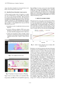
feature that allows importation of crime data from an exist- Note that Figure 5 reveals a section of raw-data information
ing file for processing (“process data” tab). (PSE) for an instance of the highlighted series. Generally,
clicking the series PDE information (that is the pie chart)
reveals the pattern space information of the corresponding
4.2. Identified Series Information Across Locations
(PDE) series at that location. The pattern space enumeration
CriClust uniquely presents cluster information in a manner (PSE) gives much more in-depth information about attribute
that can be understood by a novice public safety person- values characterising a series
nel, with no expert domain knowledge. Figure 4 presents
the identified locations with at least one series. This gives a
5. RESULTS AND DISCUSSION
quick high level insightful information on areas with repeat
offenders. However, it is worth mentioning that the map is
This paper presents a novel crime clustering model, CriClust,
able to reveal more information about the series clusters as
for crime series pattern (CSP) detection and mapping to de-
seen in Figure 5. The graduated colour map can show the
rive useful knowledge from a crime dataset. The analysis is
following for any suburb:
augmented using a dual-threshold model, and pattern preva-
lence information is encoded in similarity graphs. The sys-
• the number of series at a particular location (as seen in
tem reveals underlying strong correlations and defining fea-
Figure 4).
tures for a series, which can promote actionable knowledge.
• proportion difference evaluation (PDE) across series
identified at a specific location (i.e a pie chart with %
per series), that is the propagation effect of each series.
• pattern space enumeration (PSE), revealing attribute
information and the peculiar features that characterise
a particular series as seen in Figure 5-“Series Informa-
tion”.

Fig 6. Trend of series observed across locations with
varying data size

Furthermore, we note that when the crime records increases
the number of series identified across most of the locations
remains as it was (2 or 3 series). This means that increase
in crime record does not necessarily always imply increase
in the number of identified series at the locations or emer-
gence of a new series, as depicted in Figure 6. Table 3 de-
Fig. 4. The locations of crimes series scribes the peculiar features that characterise each series, de-
noted (S1, S2, S3). The markers “1” (presence) and “0”
(absence) respectively denote emergence or disappearance
of a corresponding feature. “Disappearance” in this con-
text means a scenario where the value of the feature is rela-
tively “undefined” or not consistent enough to be considered
as a characterising feature for the series. The emergence of
a feature does not necessarily mean that the feature has the
same “value” across all the series highlighted in Table 3 as
the opportunities available to potential offenders vary across
different spatial space. Thus having the indicator “1” for
lines (S/N) 1 and 2 for the “Day” attribute does not mean
S1 and S2 at Mowbray always happen on the same day as
they are two different series, but emerging at the same local-
ity. Furthermore, the suspect frame (SFr) attribute emerges
Fig. 5. Visualisation of series information at Wynberg for both S1 and S2 at Mowbray, but actually with unique val-
ues “moderate” and “slender” respectively. Also note that
Figure 5 shows an instance of three series identified at Wyn-
the “motivation” (Mot) feature emerges for S2 but did not
berg location, with PDEs 26 %, 34 % and 40 % respectively. emerge for S1. Hence, this feature has the indicators “0”

– 94 –